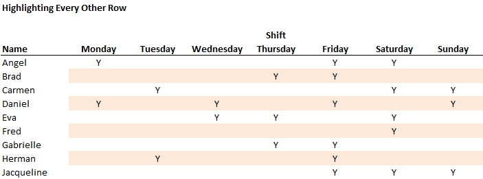
Tables are often used to layout and summarize data. But have you been in a situation where the table got so big that it is not easy to read? The table is so big that it is hard to tell which rows and columns a certain cells belong. For example, in the table below, it is hard to tell which row the “Y”‘s are starting from the 3rd row.
The Excel file with the examples used in this post: Conditional Formatting
Alternate Row Colors
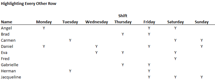
As a table gets bigger, it is easier to confuse which row or column each cell belongs to. Alternating bands of colors can make a table more intuitive and easy to read. The “Y”‘s closer to the middle is especially hard to tell which row it belongs to.
To make things more intuitive, you can use alternate shades on each row or column on the table using conditional formatting.
Below is a formula that returns true for each odd row.
=MOD(ROW(),2)=1
The conditional formatting rule shades the background of each odd row, leaving the even rows with no color. And gets something like this:
Alternate Column Colors
The same thing could be done for columns. The following line returns true for all odd columns
=MOD(COLUMN(),2)=1
In this example, data is laid out in a long table, making the 3 to 7’s hard to read. The alternating column colors make reading the table much more intuitive.
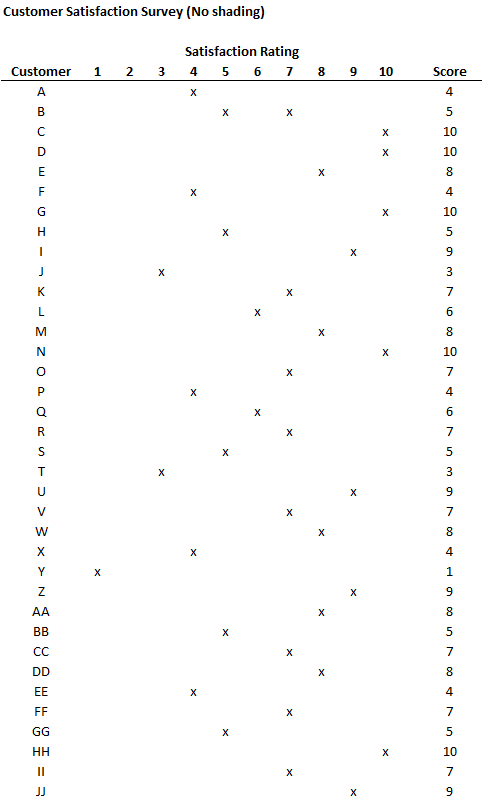
When a table has many rows, it’s hard to figure out which column the data is in, especially ones in the middle of the table.
Coloring every other column makes the table much more intuitive to read.
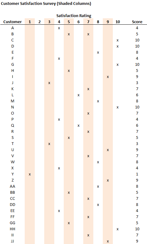
For a long table with a lot of columns, always make it easier for the reader by using conditional formatting on the columns.
Checker Patterns
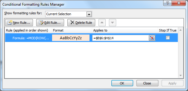
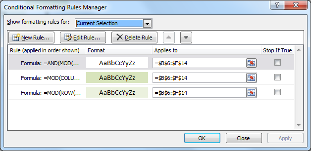
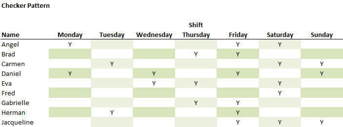
A checker pattern is a combination of alternating row and column colors, with a white cell for “intersecting” cells. Below is the conditional formatting rules window used to make the checker pattern. Note the order, the white cell format must go first:
Formulas for each corresponding conditional formatting rule:
=MOD(ROW(),2)=0,MOD(COLUMN(),2)=0)  <- selects the intersecting cell
=MOD(ROW(),2)=1  <- selects odd row
=MOD(COLUMN(),2)=1 <- selects odd columns
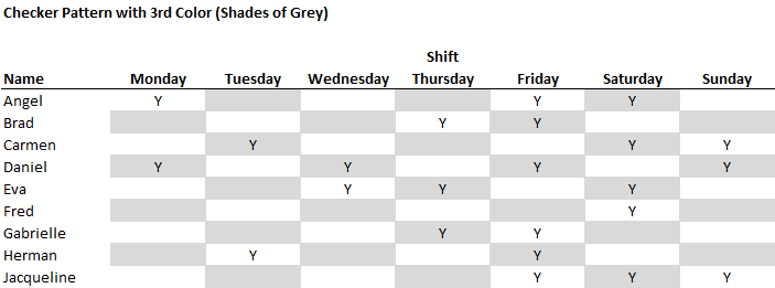
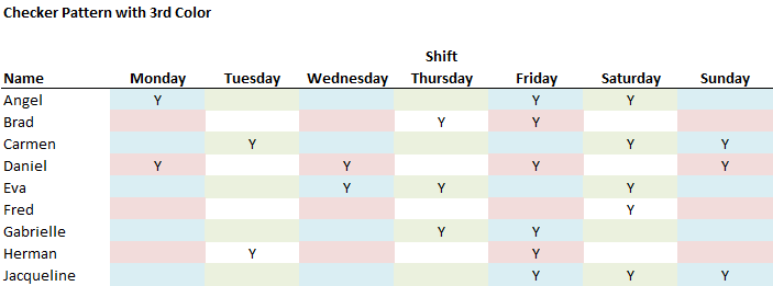
Instead of shading the intersecting cell white, a 3rd color can be used instead. In this case, blue.
You should see technique 2 in http://office.microsoft.com/en-us/excel-help/apply-shading-to-alternate-rows-in-a-worksheet-HA010251644.aspx
The checker pattern dosen’t work????