There are 2 “clean” methods to solve this problem without moving the cells:
- Excel’s filter function allows the user to filter out rows that are duplicates.
- Countif to detect any duplicates for deletion
Solution 1:
- Click on the Data -> Advanced button
- Select “Filter the list, in-place”
- For “List Range”, select the data to be filtered, in this example, column A
- Check “Unique records only”
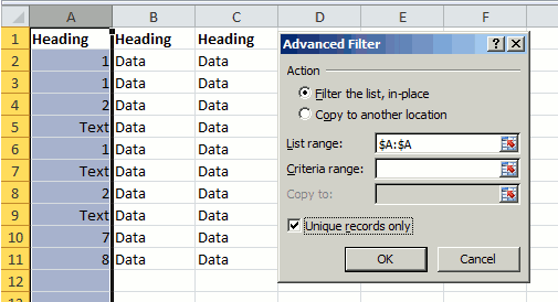
- Press OK. Only unique rows are selected
- Pick an empty column on the right (Column D in the example), type in anything on a unique row
- Copy and paste what you type till the last unique row.
- Highlight Column D and turn on the filter (In Excel 2010, its Data -> Filter button)
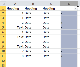
- Select only to show blank cells
- Highlight and delete rows with blank cells
- Turn off the filter – only unique cells are remaining
Solution 2:
- Find an empty column, (Column D in this example), and type in the formula
=countif([values to be sorted],[value]
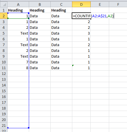
The countif function is used to count the number of times a certain value came up. If there is more than 1 match in the search area, it is a duplicate!
In this example, it is =COUNTIF(A2:A$21,A2) Note that the 2nd row reference is locked (A$21), so that no additional data will be unintentionally selected. Do not lock the row reference 1st row reference, or it will not work properly. - Copy the formula down to all rows to be filtered
- Turn on the filter on the column with the countif function
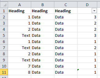
- Select all values not equal to 1
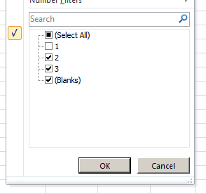
- Delete rows
- Turn off the filter – only unique cells are remaining
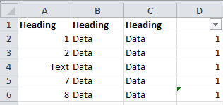
For reference, Microsoft did provide a similar solution to the problem. However, it involved copying data and deleting the original list. This seems a little more messy, because worksheets with a lot of cross referencing may have the formulas inadvertently altered. See link below: