VLOOKUP(lookup_value, table_array, col_index_num, [range_lookup])
The VLookup function can be very handy, but a few common errors throw a lot of users off. Here’s the top 5 sources of errors that I have frequently encountered over the years. Trust me, quite a few users spend hours trying to find out why the vlookup value does not work.
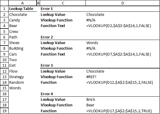
Check this screenshot of the first four type of errors, with the lookup value. The actual function is next to the “Vlookup Function” heading. The “Function Text” shows the exact formula in the “Vlookup Function” cell right above. Each error is explained in detail below. Scroll on.
Error 1 – The values look the same but Excel thinks its different!
To do a quick check to see if two values are equal, use the “=” operator. In this example, I have added an extra space ” ” behind the “Chocolate” in cell D2. So even though A2 and D2 both looks like “Chocolate”, D2 is actually “Chocolate “. Thus, the two cells are not equal in Excel.
How to check: So when in doubt, just use the = sign to quickly check if the two values are the same. The check must return TRUE, meaning Excel thinks they are equal, and for the vlookup function to work.
Error 2 – Did you select the entire table?
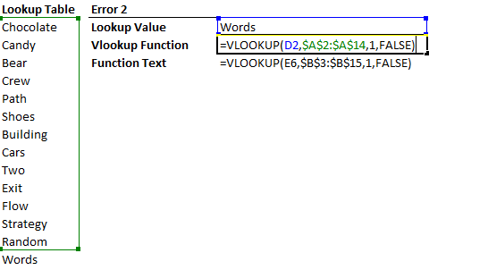
Check if the 2nd parameter, table_array, selected the entire lookup table. In this example, I (purposely) missed the last value, “Words”, in the table. Obviously, when I try to lookup “Words”, vlookup will return an error since there’s “Words” wasn’t part of the table_array.
How to check: Press F2 or look in the formula bar to see if the vlookup is looking up the entire table.
Another tip: If you have multiple vlookup cells that you copied and pasted, check at least a couple of them to see if the cell references shifted. If you want to lock in the reference to the table array (in this example A2:A14), highlight the reference press F4 once to get $A$2:$A$14.

Always check which cells are being highlighted for the lookup table. Make sure you don’t miss any parts of the table! If you are creating multiple vlookups, make sure the references are locked so the vlookup formula does not shift while copy and pasting.
Error 3 – Looking up Non-Existent Columns
Check the 3rd parameter to make sure that vlookup is looking up the right column. In this example, the table_array only has 1 column. But the formula’s third parameter (col_index_num) is 2, meaning vlookup needs to retrieve the 2nd column. Since vlookup was not supplied a 2nd column, it will return an error. To make things easier, it returns a “#REF” instead of the typical “#N/A” error.
How to check: Press F2 or look in the formula bar to see if the table you selected actually has the column number you are asking for. Notice that this is a unique error that returns a “#REF”. Meaning if you see #REF, you’ve likely to have pinpointed the problem.
Error 4 – Expecting an error, but Excel found a different match
This happens when you let Vlookup return a non-exact value, by supplying “TRUE” to the fourth parameter, range_lookup. Basically, if you left the parameter empty, or enter “FALSE”, Vlookup will either return an exact match or an error. If you enter “TRUE”, it will return either the exact value, or if the exact value does not exist, it will return the next largest value after the lookup_value, assuming the lookup table (table_array) is sorted in ascending order.
How to check: Press F2 or look in the formula bar. Ask yourself if you want an exact match or not. If you do, make sure you enter “FALSE” or leave the last parameter blank. If you do intend to get the next largest value, remember to sort the left most column of the lookup table in ascending order.
Error 5 – Circular References
When you accidentally have circular references between the lookup table, the lookup value and vlookup, it’s just the recipe for disaster (if you do not know what you are doing).
How to check: Turn off calculation for circular references. If there is a circular reference, Excel will immediately return an error. Fix accordingly to get rid of the circular reference, then turn it back on if you need it.
Error 6 – Double Entry
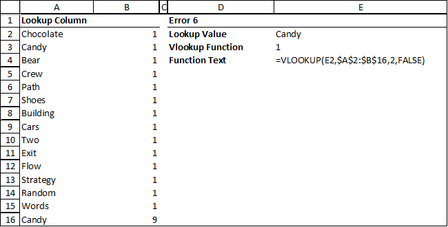
When you accidentally have a value in the lookup column entered twice (or more), but didn’t realize it. The vlookup function always looks up the first match and skips the rest. Since the values is correct, it may seem that Excel is picking up the “wrong value”.
How to check: Due a quick check to see if the value that you are looking up was already entered before.

Notice how Candy came up twice in the vlookup column (A). A user who did not know “Candy” was entered before would expect vlookup to fetch the value “9”. When there are duplicates, vlookup only shows the first match, so it returns the value “1”.
Error 7 – Floating Point Bug
Sometimes you may be looking up a column of numbers that are to be calculated. There are times where vlookup does not recognize the value due to the floating point bug. The best way is to “clean” the values in the column by using the round function. For example:
=ROUND([value],2)
How to check: This only applies to vlookup columns with values that are calculated. Check if there is indeed a rounding error. Sometimes even the check does not show problems, but vlookup still does not work. In that case, just use the round function to see if it works. See example below.

In this example, the vlookup column’s values are calculated by adding 10% to the last value. Due to a floating point bug / rounding problem, vlookup cannot find “30%” in the Lookup Column. Notice that cell D6 checks that cell A5 is equal to 30% and returns true. One of the ways to work around this bug is to use the round function. For example, =ROUND(A4+10%,2)


HELP – I am using a table that is A!:HO250. The intersections in this table represent the mileage distance between the two points. Although I am allowing for 250 rows / columns, my current needs are for only 160. I wanted to leave room for expansion. The formula finds the intersecting value when the cell reference is less than the number 258. The number 258 is not a linear number, but rather an identifying number and may represent a number that is 125 in the linear progression of numbers. I do not receive any “error” notice. I just get a “zero” value. In an effort to fix the problem, I copied the formula where it was working and pasted into a cell where it was not working. The result was the same as when I used the original formula. I will appreciate whatever assistance you are willing to give. Thanks
Error 7 isn’t mentioned in ANY other lists of vlookup errors on the internet, yet it was the one that solved my problem. THANK YOU!